游戏数据分析
在本文档中,我们分析了 VibePong 生成的游戏数据。分析内容涵盖数据提取、清洗以及带有可视化效果的探索性数据分析 (EDA)。
第一步:读取数据
首先,我们在 game_data 目录中搜索所有的摘要 (summary) 和动作 (action),遥感(telemetry) CSV 文件,并将其加载到 pandas DataFrame 中。
显示代码
import pandas as pd
import glob
import os

# 加载 game_data 目录下的所有 CSV 文件
data_dir = './game_data'
def load_combined(pattern):
    files = glob.glob(os.path.join(data_dir, f'vibepong_{pattern}_*.csv'))
    return pd.concat([pd.read_csv(f) for f in files], ignore_index=True) if files else pd.DataFrame()

df_summary = load_combined('summary')
df_actions = load_combined('actions')
df_telemetry = load_combined('telemetry')

print(f"已加载 {len(df_summary)} 行摘要数据,{len(df_actions)} 条动作记录,以及 {len(df_telemetry)} 条遥测记录。")
已加载 75 行摘要数据,366 条动作记录,以及 658 条遥测记录。
逐场游戏数据
显示代码
# Display the first few rows of summary data
df_summary.head()
| 0 |
G1770713902861-393 |
2026-02-10T08:58:27.879Z |
5.02 |
CPU |
6.56 |
light |
en |
Player 1 |
0 |
0 |
NaN |
| 1 |
G1770713902861-393 |
2026-02-10T08:58:27.879Z |
5.02 |
CPU |
6.56 |
light |
en |
CPU |
1 |
0 |
NaN |
| 2 |
G1770783544585-550 |
2026-02-11T04:20:01.889Z |
57.30 |
Player 1 |
20.38 |
dark |
en |
Player 1 |
1 |
14 |
NaN |
| 3 |
G1770783544585-550 |
2026-02-11T04:20:01.889Z |
57.30 |
Player 1 |
20.38 |
dark |
en |
CPU |
0 |
14 |
NaN |
| 4 |
G1770713913739-52 |
2026-02-10T08:58:46.511Z |
12.77 |
Player 3 |
7.08 |
light |
en |
Player 1 |
0 |
0 |
NaN |
逐个动作数据
显示代码
# Display the first few rows of summary data
df_actions.head()
| 0 |
G1770783544585-550 |
4000 |
System |
Ball served towards CPU |
NaN |
| 1 |
G1770783544585-550 |
4919 |
CPU |
Hit Ball |
NaN |
| 2 |
G1770783544585-550 |
6787 |
Player 1 |
Hit Ball |
NaN |
| 3 |
G1770783544585-550 |
8653 |
CPU |
Hit Ball |
NaN |
| 4 |
G1770783544585-550 |
10519 |
Player 1 |
Hit Ball |
NaN |
时间序列数据
显示代码
# Display the first few rows of summary data
df_telemetry.head()
| 0 |
G1770793570881-726 |
4011 |
343.50 |
349.77 |
-6.496 |
-0.2292 |
6.5010 |
20.0 |
300.0 |
350.0 |
... |
350.0 |
1.0 |
1.0 |
0.0 |
NaN |
NaN |
NaN |
NaN |
NaN |
NaN |
| 1 |
G1770793570881-726 |
4112 |
304.53 |
348.40 |
-6.496 |
-0.2292 |
6.5073 |
20.0 |
300.0 |
350.0 |
... |
350.0 |
1.0 |
1.0 |
0.0 |
NaN |
NaN |
NaN |
NaN |
NaN |
NaN |
| 2 |
G1770793570881-726 |
4227 |
259.06 |
346.79 |
-6.496 |
-0.2292 |
6.5146 |
20.0 |
300.0 |
350.0 |
... |
350.0 |
1.0 |
1.0 |
0.0 |
NaN |
NaN |
NaN |
NaN |
NaN |
NaN |
| 3 |
G1770793570881-726 |
4328 |
220.08 |
345.42 |
-6.496 |
-0.2292 |
6.5208 |
20.0 |
300.0 |
350.0 |
... |
350.0 |
1.0 |
1.0 |
0.0 |
NaN |
NaN |
NaN |
NaN |
NaN |
NaN |
| 4 |
G1770793570881-726 |
4428 |
181.11 |
344.04 |
-6.496 |
-0.2292 |
6.5271 |
20.0 |
300.0 |
350.0 |
... |
350.0 |
1.0 |
1.0 |
0.0 |
NaN |
NaN |
NaN |
NaN |
NaN |
NaN |
5 rows × 31 columns
第二步:数据清洗
我们将通过将时间戳转换为 datetime 对象、处理数值类型并确保一致性来清洗数据。
显示代码
# 清洗摘要数据
df_summary['Date'] = pd.to_datetime(df_summary['Date'])
numeric_summary = ['Duration (s)', 'Ball Speed', 'Lives', 'Hits']
df_summary[numeric_summary] = df_summary[numeric_summary].apply(pd.to_numeric, errors='coerce')
df_summary = df_summary.dropna(subset=['Player'])

# 清洗动作数据
df_actions['Timestamp (ms)'] = pd.to_numeric(df_actions['Timestamp (ms)'], errors='coerce')

df_summary.head()
| 0 |
G1770713902861-393 |
2026-02-10 08:58:27.879000+00:00 |
5.02 |
CPU |
6.56 |
light |
en |
Player 1 |
0 |
0 |
NaN |
| 1 |
G1770713902861-393 |
2026-02-10 08:58:27.879000+00:00 |
5.02 |
CPU |
6.56 |
light |
en |
CPU |
1 |
0 |
NaN |
| 2 |
G1770783544585-550 |
2026-02-11 04:20:01.889000+00:00 |
57.30 |
Player 1 |
20.38 |
dark |
en |
Player 1 |
1 |
14 |
NaN |
| 3 |
G1770783544585-550 |
2026-02-11 04:20:01.889000+00:00 |
57.30 |
Player 1 |
20.38 |
dark |
en |
CPU |
0 |
14 |
NaN |
| 4 |
G1770713913739-52 |
2026-02-10 08:58:46.511000+00:00 |
12.77 |
Player 3 |
7.08 |
light |
en |
Player 1 |
0 |
0 |
NaN |
第三步:EDA 和可视化
现在我们将查看一些关键绩效指标并可视化游戏结果。
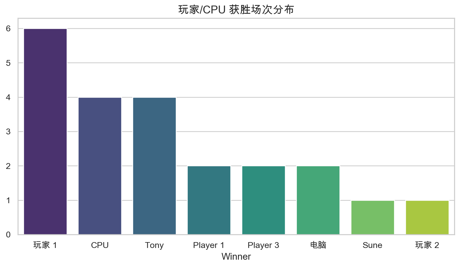
获胜分布
显示代码
import seaborn as sns
import matplotlib.pyplot as plt

# Set aesthetic style
sns.set_theme(style="whitegrid")
plt.rcParams['font.sans-serif'] = ['Arial Unicode MS']
plt.rcParams['axes.unicode_minus'] = False
谁赢得了最多的游戏?
显示代码
# 计算每位获胜者的独特游戏场次
unique_games = df_summary.drop_duplicates(subset=['Game ID'])
winner_counts = unique_games['Winner'].value_counts()

plt.figure(figsize=(10, 5))
sns.barplot(x=winner_counts.index, y=winner_counts.values, palette="viridis")
plt.title('玩家/CPU 获胜场次分布', fontsize=14)
plt.show()
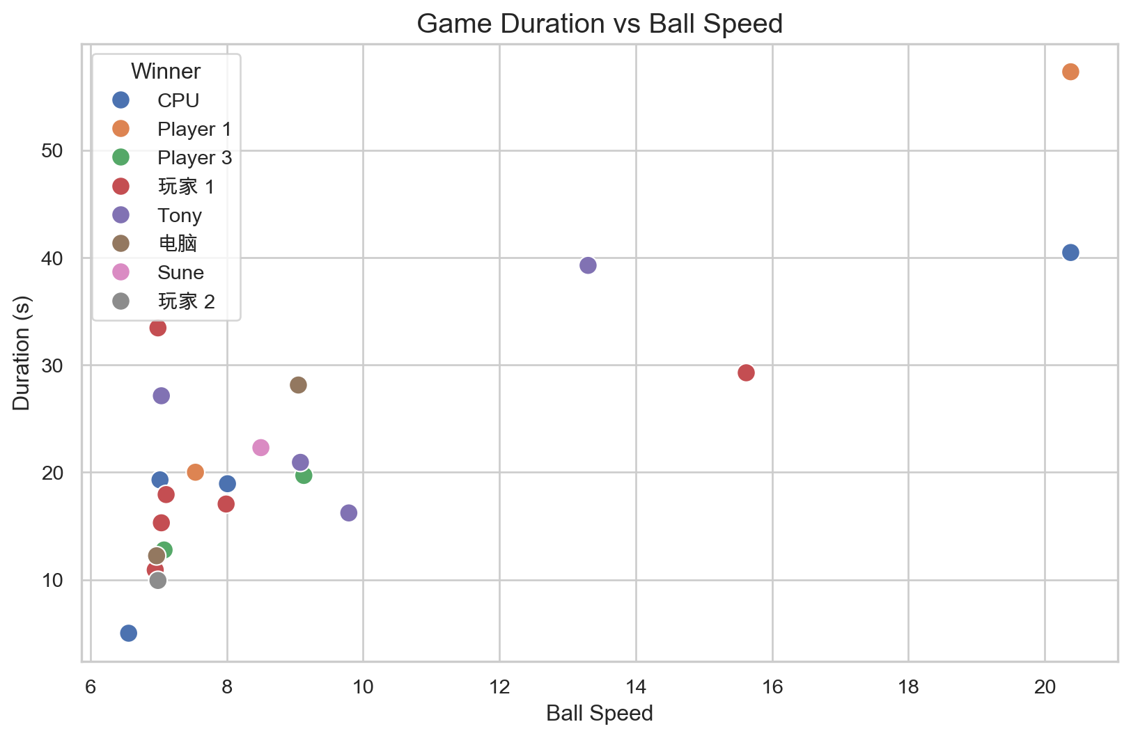
游戏时长 vs. 球速
更高的球速会导致游戏时长变短吗?
显示代码
plt.figure(figsize=(10, 6))
sns.scatterplot(data=unique_games, x='Ball Speed', y='Duration (s)', hue='Winner', s=100)
plt.title('Game Duration vs Ball Speed', fontsize=15)
plt.show()
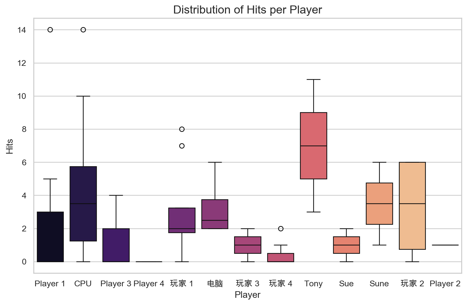
每个玩家的总击球数
跟踪不同游戏场次的技能(击球数)表现。
显示代码
plt.figure(figsize=(10, 6))
sns.boxplot(data=df_summary, x='Player', y='Hits', palette="magma")
plt.title('Distribution of Hits per Player', fontsize=15)
plt.show()
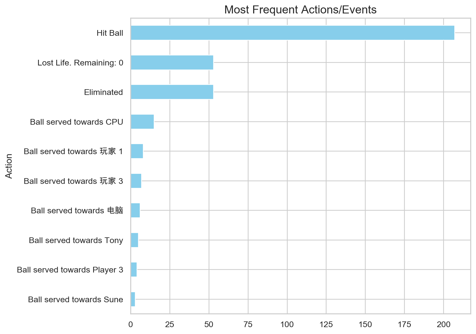
动作序列
分析所有游戏中动作的频率。
显示代码
action_counts = df_actions['Action'].value_counts().head(10)

plt.figure(figsize=(8, 7))
action_counts.plot(kind='barh', color='skyblue')
plt.title('Most Frequent Actions/Events', fontsize=15)
plt.gca().invert_yaxis()
plt.show()
第四步:遥测数据分析
现在让我们分析高频遥测数据,该数据每 100 毫秒捕获一次球和球拍的位置。
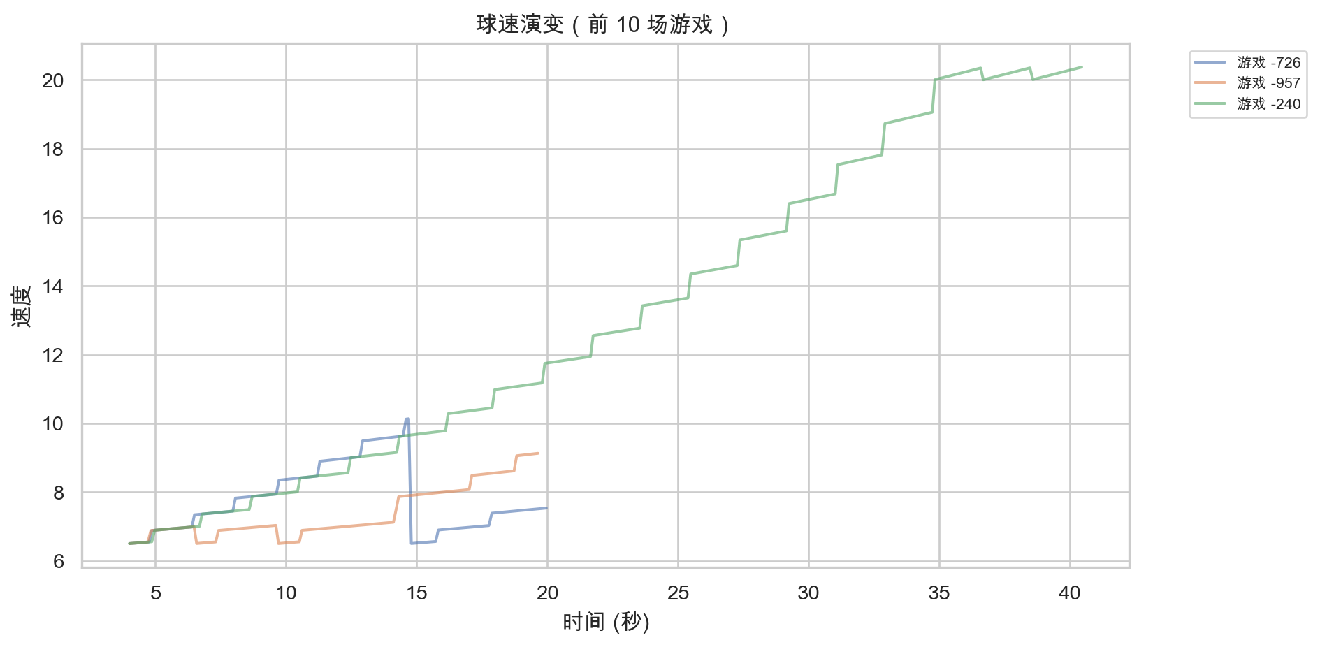
随时间变化的球速
球速在所有游戏中是如何演变的?
显示代码
if not df_telemetry.empty:
    plt.figure(figsize=(10, 5))
    for gid in df_telemetry['Game ID'].unique()[:10]:
        df_g = df_telemetry[df_telemetry['Game ID'] == gid]
        plt.plot(df_g['Timestamp (ms)']/1000, df_g['Ball Speed'], alpha=0.6, label=f'游戏 {gid[-4:]}')

    plt.title('球速演变(前 10 场游戏)')
    plt.xlabel('时间 (秒)')
    plt.ylabel('速度')
    plt.legend(bbox_to_anchor=(1.05, 1), loc='upper left', fontsize=8)
    plt.tight_layout()
    plt.show()
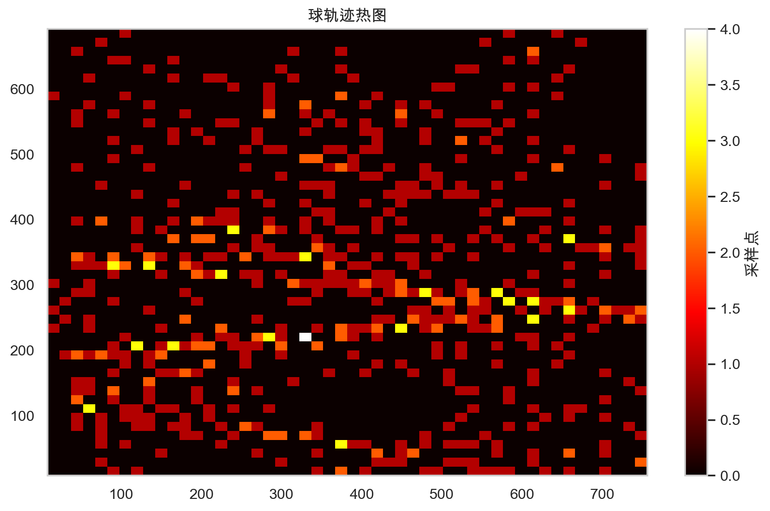
球轨迹热图
球在场地的哪个位置停留时间最长?
显示代码
if not df_telemetry.empty:
    plt.figure(figsize=(10, 6))
    plt.hist2d(df_telemetry['Ball X'], df_telemetry['Ball Y'], bins=50, cmap='hot')
    plt.colorbar(label='采样点')
    plt.title('球轨迹热图')
    plt.show()
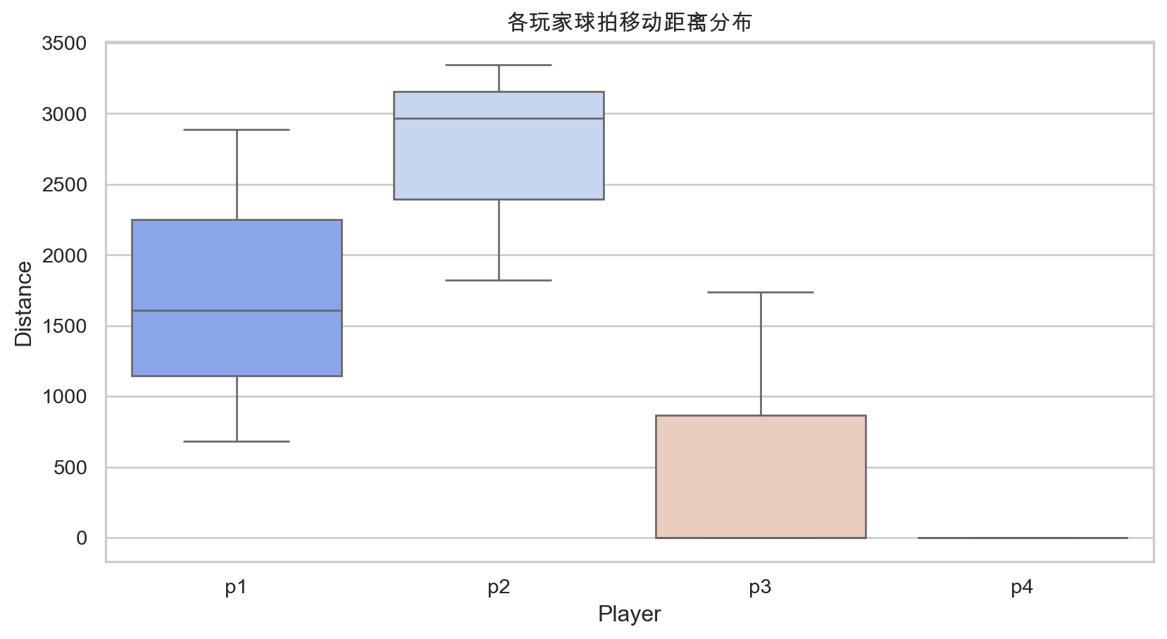
球拍移动分析
哪些玩家移动球拍最频繁?
显示代码
if not df_telemetry.empty:
    dist_cols = [c for c in df_telemetry.columns if 'Distance' in c and 'Ball' not in c]
    movement = []
    for gid in df_telemetry['Game ID'].unique():
        df_g = df_telemetry[df_telemetry['Game ID'] == gid]
        for col in dist_cols:
            movement.append({'Player': col.split()[0], 'Distance': df_g[col].sum()})

    plt.figure(figsize=(10, 5))
    sns.boxplot(data=pd.DataFrame(movement), x='Player', y='Distance', palette='coolwarm')
    plt.title('各玩家球拍移动距离分布')
    plt.show()