Vibe game:4 players Pong with game data analysis

Introduction to the game

The VibePong game is a simple yet engaging pong-style game where players can compete against each other up to 4 players or against a CPU opponent. The game features various metrics such as ball speed, game duration, and player performance, which are recorded in CSV files for analysis.

Play now :https://jcwinning.github.io/vibepong

game data analysis

In this document, we analyze the game data generated by VibePong. The analysis covers data ingestion, cleaning, and exploratory data analysis (EDA) with visualizations.

Step 1: Read Data

First, we search for all summary and action,telemetry CSV files in the game_data directory and load them into pandas DataFrames.

import pandas as pd
import glob
import os

# Load all CSV files from game_data
data_dir = './game_data'
def load_combined(pattern):
    files = glob.glob(os.path.join(data_dir, f'vibepong_{pattern}_*.csv'))
    return pd.concat([pd.read_csv(f) for f in files], ignore_index=True) if files else pd.DataFrame()

df_summary = load_combined('summary')
df_actions = load_combined('actions')
df_telemetry = load_combined('telemetry')

print(f"Loaded {len(df_summary)} summary rows, {len(df_actions)} actions, and {len(df_telemetry)} telemetry records.")

Loaded 75 summary rows, 366 actions, and 658 telemetry records.

game by game data

# Display the first few rows of summary data
df_summary.head()

	Game ID	Date	Duration (s)	Winner	Ball Speed	Theme	Language	Player	Lives	Hits	CPU Difficulty
0	G1770713902861-393	2026-02-10T08:58:27.879Z	5.02	CPU	6.56	light	en	Player 1	0	0	NaN
1	G1770713902861-393	2026-02-10T08:58:27.879Z	5.02	CPU	6.56	light	en	CPU	1	0	NaN
2	G1770783544585-550	2026-02-11T04:20:01.889Z	57.30	Player 1	20.38	dark	en	Player 1	1	14	NaN
3	G1770783544585-550	2026-02-11T04:20:01.889Z	57.30	Player 1	20.38	dark	en	CPU	0	14	NaN
4	G1770713913739-52	2026-02-10T08:58:46.511Z	12.77	Player 3	7.08	light	en	Player 1	0	0	NaN

Play by Play data

# Display the first few rows of summary data
df_actions.head()

	Game ID	Timestamp (ms)	Player	Action	Details
0	G1770783544585-550	4000	System	Ball served towards CPU	NaN
1	G1770783544585-550	4919	CPU	Hit Ball	NaN
2	G1770783544585-550	6787	Player 1	Hit Ball	NaN
3	G1770783544585-550	8653	CPU	Hit Ball	NaN
4	G1770783544585-550	10519	Player 1	Hit Ball	NaN

time by time data

# Display the first few rows of summary data
df_telemetry.head()

	Game ID	Timestamp (ms)	Ball X	Ball Y	Ball VX	Ball VY	Ball Speed	p1 X	p1 Y	p1 Center	...	p3 Center	p3 Active	p3 Lives	p3 Distance	p4 X	p4 Y	p4 Center	p4 Active	p4 Lives	p4 Distance
0	G1770793570881-726	4011	343.50	349.77	-6.496	-0.2292	6.5010	20.0	300.0	350.0	...	350.0	1.0	1.0	0.0	NaN	NaN	NaN	NaN	NaN	NaN
1	G1770793570881-726	4112	304.53	348.40	-6.496	-0.2292	6.5073	20.0	300.0	350.0	...	350.0	1.0	1.0	0.0	NaN	NaN	NaN	NaN	NaN	NaN
2	G1770793570881-726	4227	259.06	346.79	-6.496	-0.2292	6.5146	20.0	300.0	350.0	...	350.0	1.0	1.0	0.0	NaN	NaN	NaN	NaN	NaN	NaN
3	G1770793570881-726	4328	220.08	345.42	-6.496	-0.2292	6.5208	20.0	300.0	350.0	...	350.0	1.0	1.0	0.0	NaN	NaN	NaN	NaN	NaN	NaN
4	G1770793570881-726	4428	181.11	344.04	-6.496	-0.2292	6.5271	20.0	300.0	350.0	...	350.0	1.0	1.0	0.0	NaN	NaN	NaN	NaN	NaN	NaN

5 rows × 31 columns

Step 2: Data Cleaning

We will clean the data by converting timestamps to datetime objects, handling numeric types, and ensuring consistency.

# Clean Summary data
df_summary['Date'] = pd.to_datetime(df_summary['Date'])
numeric_summary = ['Duration (s)', 'Ball Speed', 'Lives', 'Hits']
df_summary[numeric_summary] = df_summary[numeric_summary].apply(pd.to_numeric, errors='coerce')
df_summary = df_summary.dropna(subset=['Player'])

# Clean Action data
df_actions['Timestamp (ms)'] = pd.to_numeric(df_actions['Timestamp (ms)'], errors='coerce')

df_summary.head()

	Game ID	Date	Duration (s)	Winner	Ball Speed	Theme	Language	Player	Lives	Hits	CPU Difficulty
0	G1770713902861-393	2026-02-10 08:58:27.879000+00:00	5.02	CPU	6.56	light	en	Player 1	0	0	NaN
1	G1770713902861-393	2026-02-10 08:58:27.879000+00:00	5.02	CPU	6.56	light	en	CPU	1	0	NaN
2	G1770783544585-550	2026-02-11 04:20:01.889000+00:00	57.30	Player 1	20.38	dark	en	Player 1	1	14	NaN
3	G1770783544585-550	2026-02-11 04:20:01.889000+00:00	57.30	Player 1	20.38	dark	en	CPU	0	14	NaN
4	G1770713913739-52	2026-02-10 08:58:46.511000+00:00	12.77	Player 3	7.08	light	en	Player 1	0	0	NaN

Step 3: EDA and Visualization

Now we’ll look at some key performance indicators and visualize the game results.

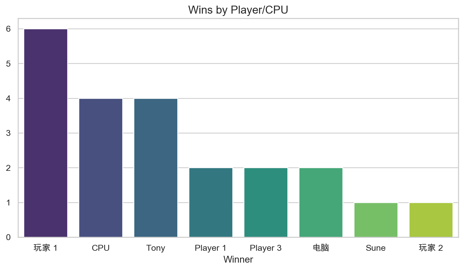
Win Distribution

import seaborn as sns
import matplotlib.pyplot as plt

# Set aesthetic style
sns.set_theme(style="whitegrid")
plt.rcParams['font.sans-serif'] = ['Arial Unicode MS']
plt.rcParams['axes.unicode_minus'] = False

Who is winning the most games?

# Count unique games per winner
unique_games = df_summary.drop_duplicates(subset=['Game ID'])
winner_counts = unique_games['Winner'].value_counts()

plt.figure(figsize=(10, 5))
sns.barplot(x=winner_counts.index, y=winner_counts.values, palette="viridis")
plt.title('Wins by Player/CPU', fontsize=14)
plt.show()

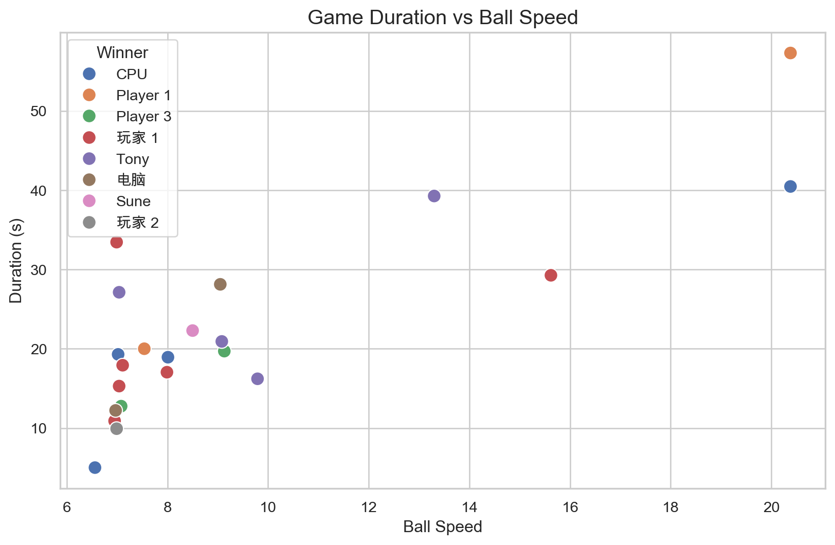
Game Duration vs. Ball Speed

Does a higher ball speed lead to shorter games?

plt.figure(figsize=(10, 6))
sns.scatterplot(data=unique_games, x='Ball Speed', y='Duration (s)', hue='Winner', s=100)
plt.title('Game Duration vs Ball Speed', fontsize=15)
plt.show()

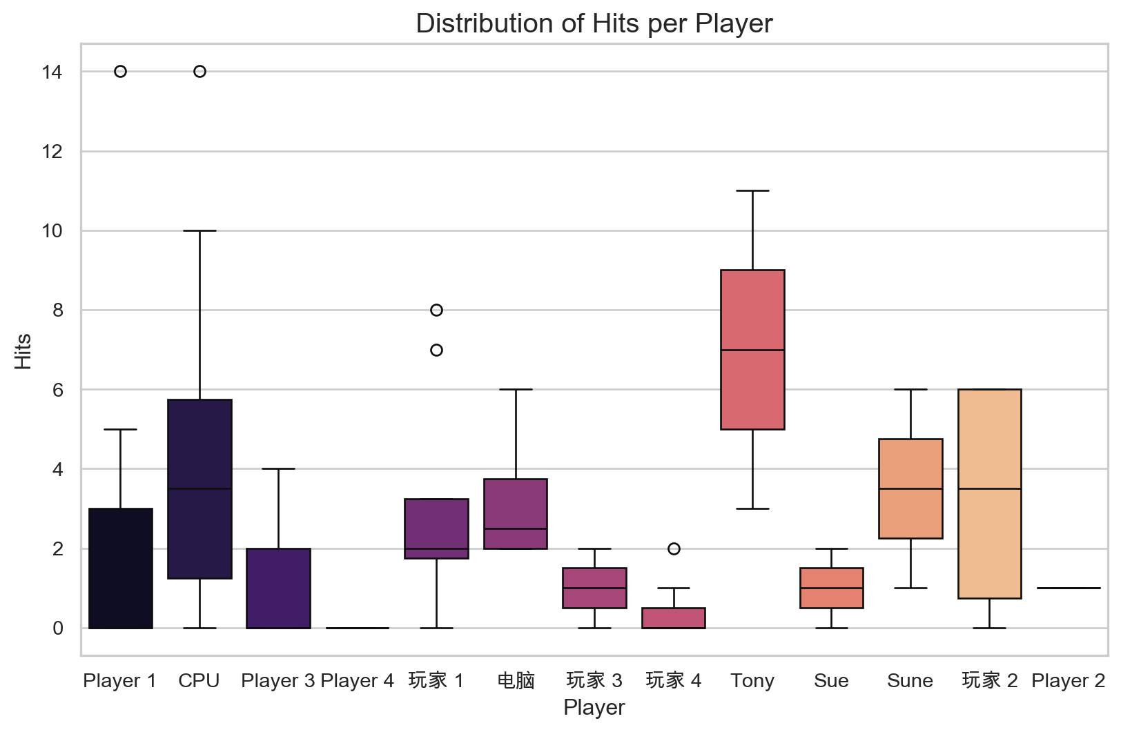
Total Hits per Player

Tracking the skill (hits) across different game sessions.

plt.figure(figsize=(10, 6))
sns.boxplot(data=df_summary, x='Player', y='Hits', palette="magma")
plt.title('Distribution of Hits per Player', fontsize=15)
plt.show()

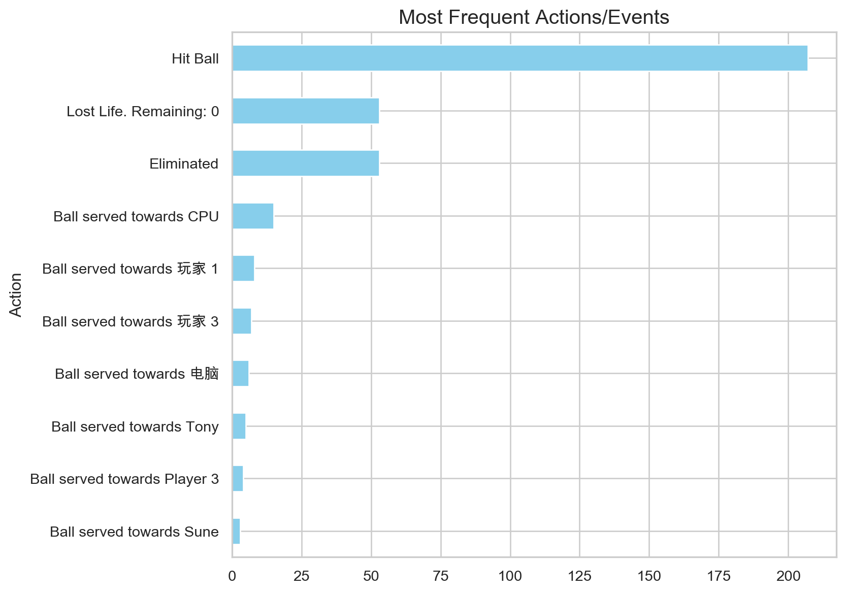
Sequence of Actions

Analyzing the frequency of actions across all games.

action_counts = df_actions['Action'].value_counts().head(10)

plt.figure(figsize=(8, 7))
action_counts.plot(kind='barh', color='skyblue')
plt.title('Most Frequent Actions/Events', fontsize=15)
plt.gca().invert_yaxis()
plt.show()

Step 4: Telemetry Data Analysis

Now let’s analyze the high-frequency telemetry data that captures ball and paddle positions every 100ms.

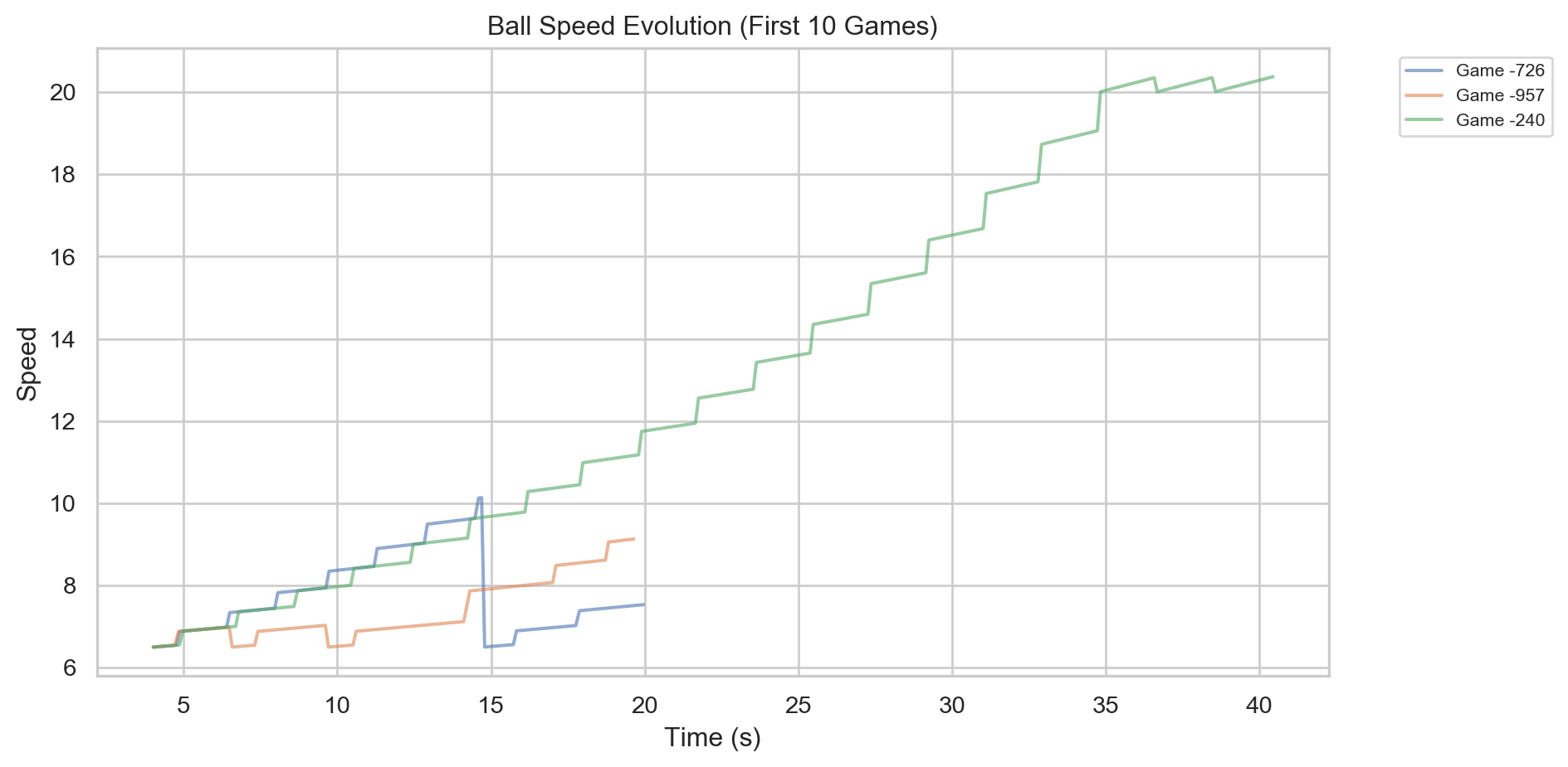
Ball Speed Over Time

How does ball speed evolve across all games?

if not df_telemetry.empty:
    plt.figure(figsize=(10, 5))
    for gid in df_telemetry['Game ID'].unique()[:10]:
        df_g = df_telemetry[df_telemetry['Game ID'] == gid]
        plt.plot(df_g['Timestamp (ms)']/1000, df_g['Ball Speed'], alpha=0.6, label=f'Game {gid[-4:]}')
    
    plt.title('Ball Speed Evolution (First 10 Games)')
    plt.xlabel('Time (s)')
    plt.ylabel('Speed')
    plt.legend(bbox_to_anchor=(1.05, 1), loc='upper left', fontsize=8)
    plt.tight_layout()
    plt.show()

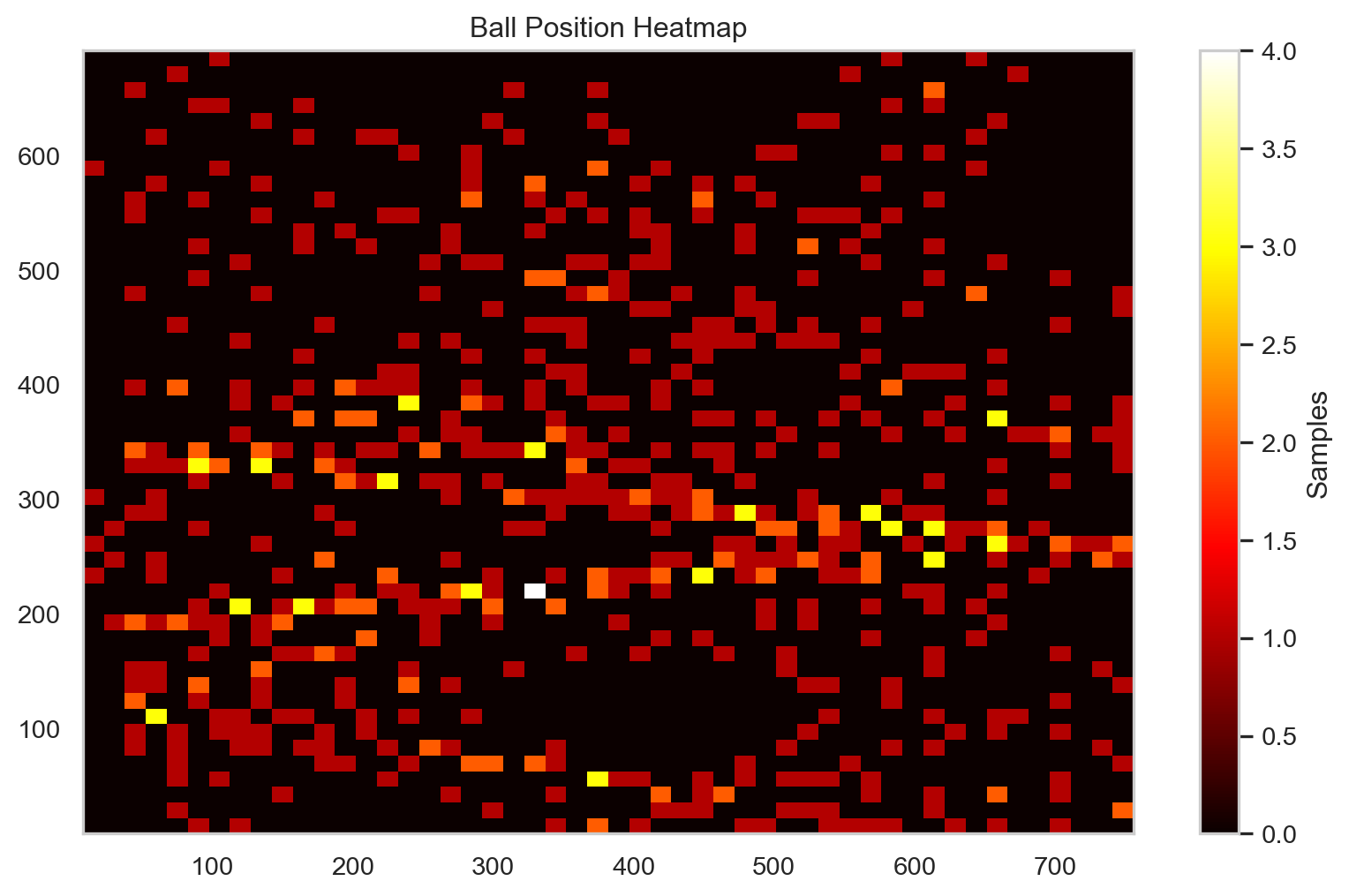
Ball Trajectory Heatmap

Where does the ball spend most of its time on the court?

if not df_telemetry.empty:
    plt.figure(figsize=(10, 6))
    plt.hist2d(df_telemetry['Ball X'], df_telemetry['Ball Y'], bins=50, cmap='hot')
    plt.colorbar(label='Samples')
    plt.title('Ball Position Heatmap')
    plt.show()

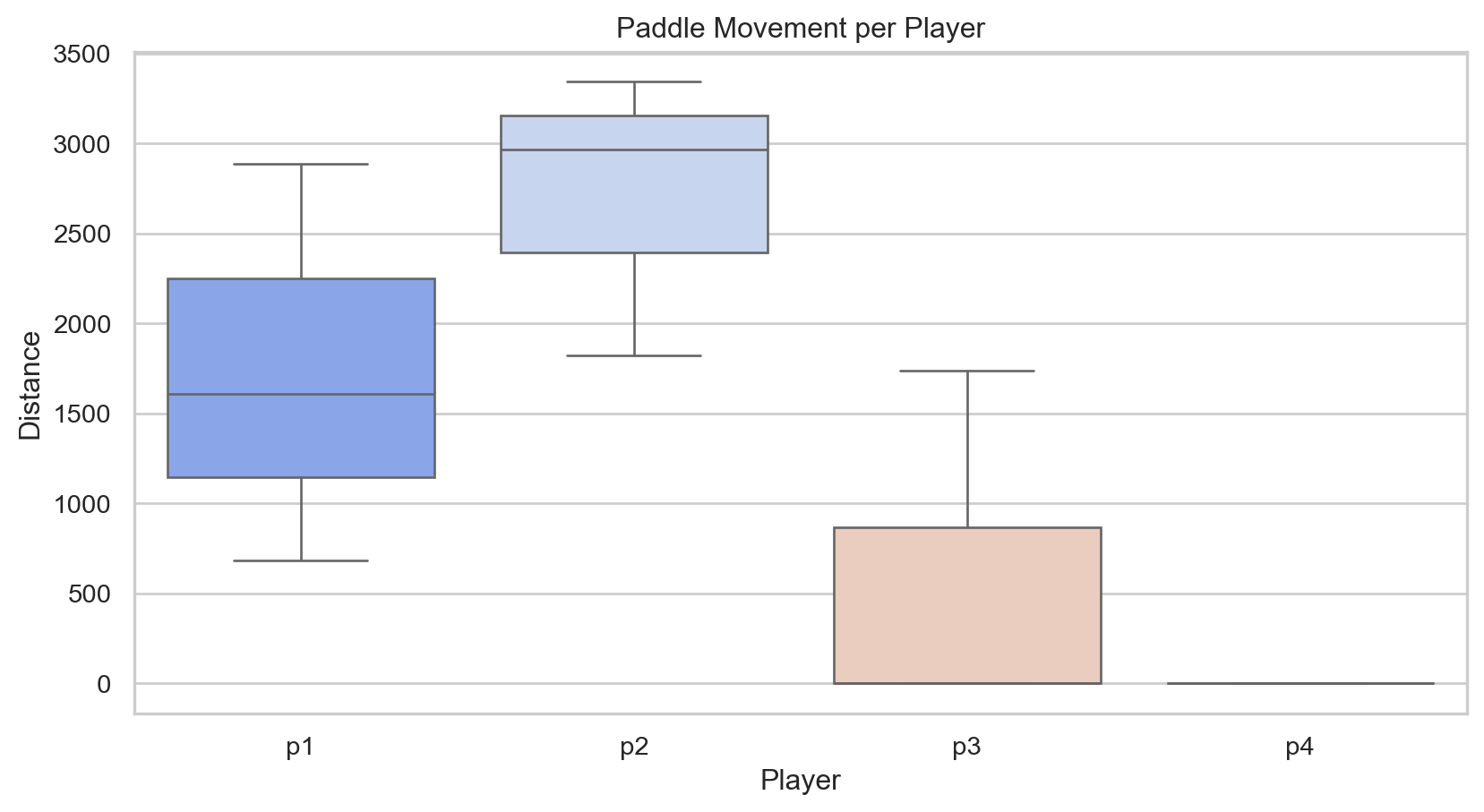
Paddle Movement Analysis

Which players move their paddles the most?

if not df_telemetry.empty:
    dist_cols = [c for c in df_telemetry.columns if 'Distance' in c and 'Ball' not in c]
    movement = []
    for gid in df_telemetry['Game ID'].unique():
        df_g = df_telemetry[df_telemetry['Game ID'] == gid]
        for col in dist_cols:
            movement.append({'Player': col.split()[0], 'Distance': df_g[col].sum()})
    
    plt.figure(figsize=(10, 5))
    sns.boxplot(data=pd.DataFrame(movement), x='Player', y='Distance', palette='coolwarm')
    plt.title('Paddle Movement per Player')
    plt.show()